Cross-Entropy
This post is the second in a series of two, the first looking at entropy. Cross-entropy is a common loss function in machine learning and is a little less intuitive than something like mean squared error, so I wrote this post to help clarify things for myself and colleagues at the time.
As we saw in an earlier post, entropy is calculated as follows: $$H(p) = -\sum_{x} p(x)\log_{2} p(x)$$ Looking at the above formula, you might wonder, “what would happen if we were to replace the $p(x)$ in $\log_{2} p(x)$ with another pmf?” That is, we would now be looking at the expectation of $\log_{2}q(x)$ while retaining the probability distribution $x\sim p$.
Note: You may notice that I am defining entropy using $\log$ with base 2, rather than leaving the base aribtrary. Base 2 is natural when we are thinking of encoding messages in binary, but the properties of entropy do not depend on having a base of 2, so any other base can be used, including, for mathematicians, the more natural $\ln$. The proper defintion of entropy does not include the base of 2.
Going back to our original motivation for entropy, this means we would be asking “what is the average length of a message using an encoding $q(x)$ if the content of that message is distributed like $p(x)$?”
Remember that since we are talking about encoding in binary, we are looking at length of messages in bits, so the encoding size is $–log_{2}q = log_{2}(1/q)$.
Mathematically, we are asking for this quantity: $$H(p, q) = -\sum_{x} p(x)\log_{2} q(x)$$
Encoding messages with a length equal to their probability gives you the optimal encoding length; that is, entropy is a measure of the optimal average encoding length. Hence, if $q \ne p$, then we have a suboptimal encoding length for our messages. Cross-entropy can therefore be seen as the average length of communicating an event from one probability distribution with the optimal encoding of another probability distribution.
Note that cross-entropy is not symmetric, so $H(p, q)$ does not necessarily equal $H(q, p)$. The following example makes this clear.
Imagine that we have two individuals, call them Amir and Melody, who communicate with each other. The only messages Amir and Melody communicate are "Excellent", "Good", "Bad", "Terrible". Hey, not everyone is a great conversationalist. Amir and Melody communicate these messages with the following frequencies:
| Message | Amir ($p(x)$) | Melody ($q(x)$) |
|---|---|---|
| Excellent | $1/2$ | $1/8$ |
| Good | $1/4$ | $1/2$ |
| Bad | $1/8$ | $1/4$ |
| Terrible | $1/8$ | $1/8$ |
As we can see from the table, Amir has a probability distribution $p(x)$ over the space of messages, and Melody has a probability distribution $q(x)$ over the space of messages. Using this $p$ and $q$, we can calculate entropy and cross-entropy.
$$\begin{split} H(p) &= -\sum p(x)\log_2 p(x) \\ &= -(1/2 \cdot \log_2(1/2) + 1/4 \cdot \log_2(1/4) + 1/8 \cdot \log_2(1/8) + 1/8 \cdot \log_2(1/8)) \\ &= -((-1/2) - 1/2 - 3/8 - 3/8) \\ &= 1.75 \end{split}$$
$$\begin{split} H(q) &= -\sum q(x)\log_2 q(x) \\ &= -(1/8 \cdot \log_2(1/8) + 1/2 \cdot \log_2(1/2) + 1/4 \cdot \log_2(1/4) + 1/8 \cdot \log_2(1/8)) \\ &= -((-3/8) - 1/2 - 1/2 - 3/8) \\ &= 1.75 \end{split}$$
$$\begin{split} H(p, q) &= -\sum p(x)\log_2 q(x) \\ &= -(1/2 \cdot \log_2(1/8) + 1/4 \cdot \log_2(1/2) + 1/8 \cdot \log_2(1/4) + 1/8 \cdot \log_2(1/8)) \\ &= -((-3/2) - 1/4 - 1/4 - 3/8) \\ &= 2.375 \end{split}$$
$$\begin{split} H(q, p) &= -\sum q(x)\log_2 p(x) \\ &= -(1/8 \cdot \log_2(1/2) + 1/2 \cdot \log_2(1/4) + 1/4 \cdot \log_2(1/8) + 1/8 \cdot \log_2(1/8)) \\ &= -((-1/8) - 1 - 3/4 - 3/8) \\ &= 2.25 \end{split}$$
So, as we can see, while $H(p)$ is equal to$ H(q)$, $H(p, q)$ is not equal to $H(q, p)$.
| $H(p)$ | $H(q)$ | $H(p,q)$ | $H(q,p)$ |
|---|---|---|---|
| 1.75 | 1.75 | 2.375 | 2.25 |
In this example, what we are asking when calculate cross-entropy is "what is the average message length if Amir encodes his messages with lengths chosen according Melody's message frequencies, and vice versa?". In this case it is actually more expensive for Amir to encode his messages according to Melody's probability distribution than it is for Melody to encode her messages according to Amir's probability distribution.
Entropy vs Cross-Entropy
Since entropy represents the average length of the optimal encoding, it should be the case that cross-entropy is always greater than or equal to entropy, with equality being achieved if and only if $p = q$. That is: $$H(p,q) \ge H(p)$$ This is indeed true, and we will prove it shortly, but first we will introduce another concept that we will use in the proof.
If we compare $H(p, q)$ to $H(p)$, it could be interesting to see how much they differ in magnitude. The difference between the two reflects how much longer messages would be if you used an encoding system optimized for a different probability distribution. This should give us some measure of how different two probability distributions are from each other. Clearly, if $p = q$ then $H(p, q) = H(p)$, but the more different $p$ and $q$ are, the more $H(p, q)$ and $H(p)$ should diverge.
Unsurprisingly, this concept is well-defined and is known as Kullback-Leibler divergence (usually referred to as KL divergence). KL divergence is defined as $$D_{KL}(P\parallel Q) = H(p, q) – H(p)$$ This is actually not the standard definition of KL divergence, but if we manipulate the above expression we get the usual definition for KL divergence
$$\begin{split} D_{KL}(P\parallel Q) &= H(p, q) – H(p) \\ &= -\sum_{x} p(x)\log_{2} q(x) + \sum_{x} p(x)\log_{2} p(x) \\ &= \sum_{x} p(x)(\log_{2} p(x) - \log_{2} q(x)) \\ &= \sum_{x} p(x)\log_{2}\left({\frac {p(x)}{q(x)}}\right) \\ &= -\sum_{x} p(x)\log_{2}\left({\frac {q(x)}{p(x)}}\right) \end{split}$$
Now that we’ve defined KL divergence, we can proceed with the proof that $$H(p, q) \ge H(p)$$ Since $D_{KL}(P\parallel Q) = H(p, q) – H(p)$, if we can show $D_{KL}(P\parallel Q) \ge 0$ then we have our desired result. In fact, we’ll show that $-D_{KL}(P\parallel Q) \le 0$, which obviously gives us $D_{KL}(P\parallel Q) \ge 0$. There are many ways to get this proof,
$$\begin{split} -D_{KL}(P\parallel Q) &= -\sum_x p(x)\log_{2} \left({\frac {p(x)}{q(x)}}\right)\\ &= \sum_x p(x)\log_{2} \left({\frac {p(x)}{q(x)}}\right)\\ &\stackrel{\text{(*)}}{\leq} \log_2 \sum_x p(x)\left({\frac {q(x)}{p(x)}}\right)\\ &=\log_{2} 1\\ &=0 \end{split}$$
The inequality step at (*) uses Jensen’s inequality and the fact that log is a concave function. We won’t prove Jensen’s inequality here, but we will at least state it for the sake of completeness (the proof is actually quite simple for the finite form and can be shown using induction). Jensen’s inequality (finite form):
Jensen's Inequality: Let $p_1, ..., p_n$ be positive numbers such that $\sum_{i=1}^{n}p_i = 1$ and let $f$ be a real continuous function that is convex, then $$f\left(\sum_{i=1}^{n}p_ix_i \right) \le \sum_{i=1}^{n}p_i f(x_i).$$
Just in case you're not familiar with convex functions, we'll state the definition here:
Definition (Convex Function): Consider a function $g: I \rightarrow \mathbb{R}$, where $I$ is an interval in $\mathbb{R}$. We say that $g$ is a convex function if, for any two points $x$ and $y$ in $I$ and any $\alpha\in[0,1]$, we have $$g(\alpha x+ (1-\alpha)y) \leq \alpha g(x)+ (1-\alpha)g(y).$$
As you can see, Jensen's inequality merely extends the definition of a convex function to an arbitrary finite number of points. If you've never seen the definition of a convex function before, it may look a bit confusing, but all it says is that if you draw a secant line connecting two points on the curve of a convex function, the line will lie on or above the curve described by the convex function. This is easily visualized.
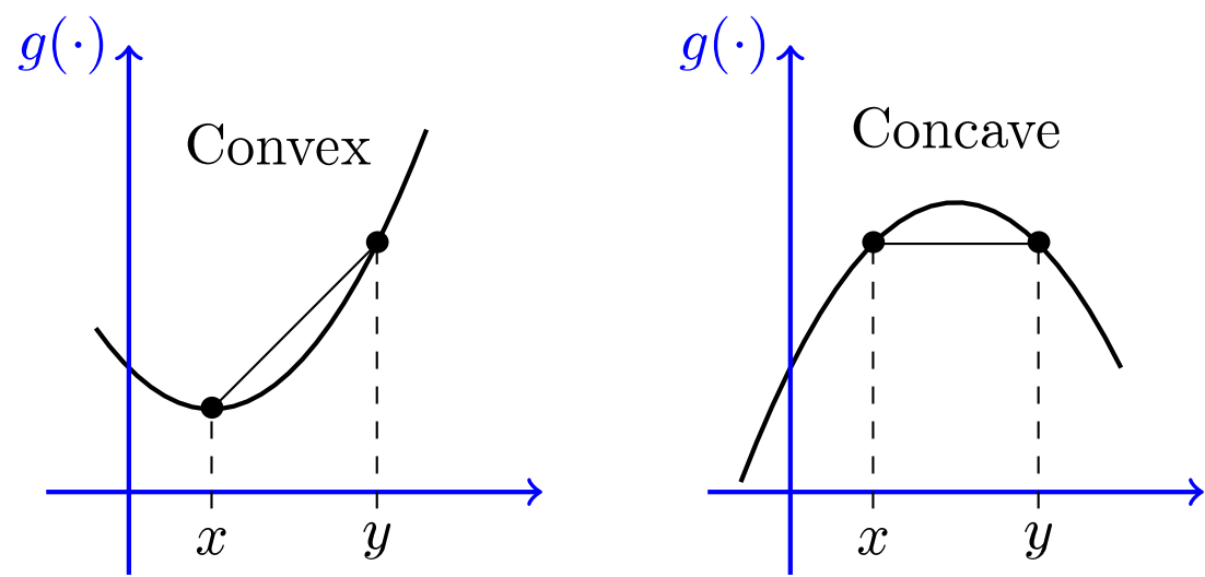 A convex function and a concave function.
If you found that proof confusing, don't worry about it; you don't need to understand the details to get the important pieces. The really important takeaway here is that cross-entropy is always greather than or equal to entropy, with equality achieved if and only if the two distributions are equal. It's this notion - cross-entropy providing some kind of measure for the distance of probability distributions from each other - that is really useful for machine learning.
Cross-Entropy as a loss function
I think the notion of cross-entropy as a loss function is best illustrated with an example, so we'll start with that.
Imagine we have classification task with 4 potential output categories we'll call A, B, C, and D (think image classification into cat, dog, horse, bird if that helps). Each data-point (image) is labelled according to the category they belong to. This label can be represented using one-hot encoding.
| Category | Encoding |
|---|---|
| A | $[1\ 0\ 0\ 0]$ |
| B | $[0\ 1\ 0\ 0]$ |
| C | $[0\ 0\ 1\ 0]$ |
| D | $[0\ 0\ 0\ 1]$ |
This one-hot encoding actually defines a probability distribution over the data-points. For example if a data-point, say $x_4$, has one-hot encoding $x_4 = [0\ 1\ 0\ 0]$ ,then $x_4$ has a probability of $1$ of being from category B and and zero probability of being from another category. $$\begin{split} P_{x_4}(A) &= 0 \\ P_{x_4}(B) &= 1 \\ P_{x_4}(C) &= 0 \\ P_{x_4}(D) &= 0 \\ \end{split}$$
I realize this is weird notation, but $P_{x_4}(i)$ here just means the probability of $x_4$ of belonging to the $i$th category. Maybe another point, $x_{16}$ has one-hot encoding $x_{16} = [1\ 0\ 0\ 0]$, meaning $x_{16}$ belongs to category A. Hence, $$\begin{split} P_{x_{16}}(A) &= 1 \\ P_{x_{16}}(B) &= 0 \\ P_{x_{16}}(C) &= 0 \\ P_{x_{16}}(D) &= 0 \\ \end{split}$$
What if we calculate the entropy of one of these data-points? $$\begin{split} H(P_{x_4}) &= -\sum P_{x_4}(i)\log P_{x_4}(i) \\ &= -(0 \cdot \log(0) + 1 \cdot \log(1) + 0 \cdot \log(0) + 0 \cdot \log(0)) \\ &= -(0 + 0 + 0 + 0) \\ &= 0 \end{split}$$
This is clearly true for all data-points with one-hot encodings, so they all have zero entropy. This makes sense as there is no uncertainty or surprise involved - each data-point belongs to a category with probability equal to 1. Now imagine we train a model to predict the categories of our data-points. The output vector we obtain when we feed-forward through the trained model also defines a probability distribution over our categories. Let's call these output vectors $Q_{x_i}$, and say that $Q_{x_4} = [0.2\ 0.6\ 0.15\ 0.05]$.
Now we have two different probability distributions over the data-point - the real distribution, and the distribution predicted by our model - so we can calculate the cross-entropy between the distributions. I will use the natural logarithm, $\ln$, for these calculations. $$\begin{split} H(P_{x_4}, Q_{x_4}) &= -\sum P_{x_4}(i)\log Q_{x_4}(i) \\ &= -(0 \cdot \log(0.2) + 1 \cdot \log(0.6) + 0 \cdot \log(0.15) + 0 \cdot \log(0.05)) \\ &= -(0 - 0.511 + 0 + 0) \\ &\approx 0.511 \end{split}$$
As expected, this is higher than the entropy for $x_4$ because, as discussed earlier, cross-entropy is always greater than or equal to entropy. What would happen if we trained our model for longer, and got a better prediction? Let's say the prediction from our improved model is $Q^{\prime}_{x_4} = [0.01\ 0.98\ 0.005\ 0.005]$. In this case our cross-entropy claculation gives us $$\begin{split} H(P_{x_4}, Q^{\prime}_{x_4}) &= -\sum P_{x_4}(i)\log Q_{x_4}(i) \\ &= -(0 \cdot \log(0.01) + 1 \cdot \log(0.98) + 0 \cdot \log(0.005) + 0 \cdot \log(0.005)) \\ &= -(0 - 0.0202 + 0 + 0) \\ &\approx 0.0202 \end{split}$$
As our prediction improves, that is as $Q^{\prime}_{x_4}$ gets closer to $P_{x_4}$, cross-entropy decreases. In other words, as the predicted distribution approaches the real distribution, cross-entropy approaches entropy.
As we can see from this example, as our predicted distributions begin to approach the real distribution, the value of the cross-entropy decreases. So if we are using a cross-entropy loss function, we will minimize our model's loss as the predictions approach the real value, something we obviously desire.
It's worth quickly mentioning why I used $\ln$ instead of $\log_2$ for the calculations. In machine learning we use base $e$ instead of base 2 for a few reasons, one of which is that it is typically faster to calculate $\ln$ using a computer. This may seem strange given that we motivated our entire discussion of entropy by talking about encoding messages in binary, but for the purposes of a machine learning loss function there is no necessity to use base 2, and as $\log_2(x) = {\frac {\ln(x)}{\ln(2)}}$ the two differ only by a constant factor anyways.
This example made use of cross-entropy as a loss function for a classification problem, but there are other types of machine learning models where cross-entropy is useful, and perhaps an even more natural fit. GANs (Generative Adversarial Networks) are a prime example of this. In a GAN, the generator network is trying to learn the probability distribution of the real data and the discriminator network is trying distinguish between data points that were generated from the real data versus the generator network. The entire goal of GANs hinges on learning to replicate a latent probability distribution, so it is very natural to use a measure of distance or difference between probability distributions such as cross-entropy as a loss function.
If you've seen cross-entropy loss functions used in machine learning, chances are you've also come across binary cross-entropy before. Binary cross-entropy isn't anything new from what we've discussed so far, rather it is just a special formulation of cross-entropy for a binary problem (hence the name), i.e. 0 or 1, yes or no. If you are predicting just two categories - we'll use "yes" and "no" - then your cross-entropy looks like this $$\begin{split} H(P, Q) &= -\sum_{i \in (yes,\ no)} P(i)\log Q(i) \\ &= -(P(yes)\log Q(yes) + P(no)\log Q(no)) \end{split}$$
Since we only have two categories here though, we have $$P(no) = (1 - P(yes)) \ \ \ and\ \ \ Q(no) = (1 - Q(yes))$$ Hence our cross-entropy can be written as follows $$H(P, Q) = -(P(yes)\log Q(yes)) + (1 - P(yes))\log (1 - Q(yes))$$
There are further concepts in information theory that are both fascinating, and of great importance in machine learning, that are well worth digging into. Some terms to check out for those curious are: mutual information, Jensen-Shannon divergence, joint entropy, and conditional entropy.
I should also note that like most mathematical concepts, entropy and cross-entropy are remarkably multi-faceted and can be looked at from a wide variety of different perspectives. I've tried to give an explanation that is useful for me in building intuition, but there are also ways to think about cross-entropy in machine learning from a Bayesian perspective for example. I am also not an expert in information theory by any means, so it is likely I've missed some important points in my explanation. That being said, I hope it helps to provide some intuition for what is going on in the sometimes esoteric looking sums involving $P$s, $Q$s and $log$s.
In case you missed it, the first post in these series of two introduces the notion of entropy.